Soil microbiome networks

Microbial abundance networks are a typical application of Graphical Lasso. [ref12]

We have a look at a dataset of 88 soil samples from North and South America. We do two steps of preprocessing:

• We filter on OTUs with a minimum frequeny of 100, obtaining \(N=88\) samples of counts from \(p=116\) OTUs.

• We replace zero counts by adding a pseudocount of 1 to all entries.

Bacterial composition is correlated with environmental variables, such as temperature, moisture or pH. In this experiment, we want to demonstrate that these confounding factors can be reconstructed using Graphical Lasso with latent variables.

# sphinx_gallery_thumbnail_number = 2

import numpy as np
import pandas as pd

import seaborn as sns
import matplotlib.pyplot as plt
from scipy import stats

from gglasso.helper.utils import sparsity, zero_replacement, normalize, log_transform
from gglasso.problem import glasso_problem
from gglasso.helper.basic_linalg import scale_array_by_diagonal

For this, we first load the dataset and compute relative abundances (this is done by normalize). Hence, we obtain compositional data where each sample is on the unit simplex. Typically, Graphical Lasso is not applied to compositional data directly. We apply the centered log-ratio transform (using log_transform).

soil = pd.read_csv('../data/soil/processed/soil_116.csv', sep=',', index_col = 0).T
print(soil.head())

X = normalize(soil)

X = log_transform(X)
(p,N) = X.shape

print("Shape of the transformed data: (p,N)=", (p,N))

         103.CA2  103.CO3  103.SR3  103.IE2  ...  103.AR1  103.TL1  103.HI4  103.BB1
1124701     16.0     15.0      2.0      9.0  ...      1.0      1.0      1.0      1.0
697997       3.0      5.0      1.0      1.0  ...      1.0      1.0      1.0      1.0
203969       1.0      1.0      1.0      1.0  ...      1.0      1.0      1.0      1.0
205391       1.0      1.0      1.0      2.0  ...      1.0      7.0      1.0      1.0
843189       1.0      1.0      1.0      1.0  ...      1.0      2.0      2.0      1.0

[5 rows x 89 columns]
Shape of the transformed data: (p,N)= (116, 89)

The dataset also contains the pH value for each sample. We do not make use of this for estimating the network. We also calculate the sampling depth, i.e. the number of total counts per sample.

ph = pd.read_csv('../data/soil/processed/ph.csv', sep=',', index_col = 0)
ph = ph.reindex(soil.columns)
print(ph.head())

depth = soil.sum(axis=0)

metadata = pd.read_table('../data/soil/original/88soils_modified_metadata.txt', index_col=0)

temperature = metadata["annual_season_temp"].reindex(ph.index)

           ph
103.CA2  8.02
103.CO3  6.02
103.SR3  6.95
103.IE2  5.52
103.BP1  7.53

We compute the empirical covariance matrix and scale it to correlations. Then, we create an instance of glasso_problem and do model selection using a grid search. Note that we set latent=True because we want to account for unobserved latent factors.

S0 = np.cov(X.values, bias = True)
S = scale_array_by_diagonal(S0)


P = glasso_problem(S, N, latent = True, do_scaling = False)
print(P)

lambda1_range = np.logspace(0.5,-1.5,8)
mu1_range = np.logspace(1.5,-0.2,6)

modelselect_params = {'lambda1_range': lambda1_range, 'mu1_range': mu1_range}

P.model_selection(modelselect_params = modelselect_params, method = 'eBIC', gamma = 0.25)

print(P.reg_params)

SINGLE GRAPHICAL LASSO PROBLEM WITH LATENT VARIABLES
Regularization parameters:
{'lambda1': None, 'mu1': None}
ADMM terminated after 38 iterations with status: optimal.
ADMM terminated after 41 iterations with status: optimal.
ADMM terminated after 26 iterations with status: optimal.
ADMM terminated after 25 iterations with status: optimal.
ADMM terminated after 57 iterations with status: optimal.
ADMM terminated after 61 iterations with status: optimal.
ADMM terminated after 34 iterations with status: optimal.
ADMM terminated after 41 iterations with status: optimal.
ADMM terminated after 26 iterations with status: optimal.
ADMM terminated after 25 iterations with status: optimal.
ADMM terminated after 57 iterations with status: optimal.
ADMM terminated after 61 iterations with status: optimal.
ADMM terminated after 34 iterations with status: optimal.
ADMM terminated after 41 iterations with status: optimal.
ADMM terminated after 26 iterations with status: optimal.
ADMM terminated after 25 iterations with status: optimal.
ADMM terminated after 57 iterations with status: optimal.
ADMM terminated after 61 iterations with status: optimal.
ADMM terminated after 126 iterations with status: optimal.
ADMM terminated after 53 iterations with status: optimal.
ADMM terminated after 27 iterations with status: optimal.
ADMM terminated after 24 iterations with status: optimal.
ADMM terminated after 57 iterations with status: optimal.
ADMM terminated after 61 iterations with status: optimal.
ADMM terminated after 148 iterations with status: optimal.
ADMM terminated after 149 iterations with status: optimal.
ADMM terminated after 52 iterations with status: optimal.
ADMM terminated after 38 iterations with status: optimal.
ADMM terminated after 56 iterations with status: optimal.
ADMM terminated after 62 iterations with status: optimal.
ADMM terminated after 95 iterations with status: optimal.
ADMM terminated after 66 iterations with status: optimal.
ADMM terminated after 66 iterations with status: optimal.
ADMM terminated after 58 iterations with status: optimal.
ADMM terminated after 55 iterations with status: optimal.
ADMM terminated after 62 iterations with status: optimal.
ADMM terminated after 116 iterations with status: optimal.
ADMM terminated after 53 iterations with status: optimal.
ADMM terminated after 53 iterations with status: optimal.
ADMM terminated after 53 iterations with status: optimal.
ADMM terminated after 63 iterations with status: optimal.
ADMM terminated after 82 iterations with status: optimal.
ADMM terminated after 126 iterations with status: optimal.
ADMM terminated after 55 iterations with status: optimal.
ADMM terminated after 56 iterations with status: optimal.
ADMM terminated after 56 iterations with status: optimal.
ADMM terminated after 56 iterations with status: optimal.
ADMM terminated after 84 iterations with status: optimal.
{'lambda1': 0.22758459260747887, 'mu1': 6.606934480075961}

The Graphical Lasso solution is of the form \(\Theta - L\) where \(\Theta\) is sparse and \(L\) has low rank. We use the low rank component of the Graphical Lasso solution in order to do a robust PCA. For this, we use the eigendecomposition

\[L = V \Sigma V^T\]

where the columns of \(V\) are the orthonormal eigenvecors and \(\Sigma\) is diagonal containing the eigenvalues. Denote the columns of \(V\) corresponding only to positive eigenvalues with \(\tilde{V} \in \mathbb{R}^{p\times r}\) and \(\tilde{\Sigma} \in \mathbb{R}^{r\times r}\) accordingly, where \(r=\mathrm{rank}(L)\). Then we have

\[L = \tilde{V} \tilde{\Sigma} \tilde{V}^T.\]

Now we project the data matrix \(X\in \mathbb{R}^{p\times N}\) onto the eigenspaces of \(L^{-1}\) - which are the same as of \(L\) - by computing

\[U := X^T \tilde{V}\tilde{\Sigma}.\]

def robust_PCA(X, L, inverse=True):
    sig, V = np.linalg.eigh(L)

    # sort eigenvalues in descending order
    sig = sig[::-1]
    V = V[:,::-1]

    ind = np.argwhere(sig > 1e-9)

    if inverse:
        loadings = V[:,ind] @ np.diag(np.sqrt(1/sig[ind]))
    else:
        loadings = V[:,ind] @ np.diag(np.sqrt(sig[ind]))

    # compute the projection
    zu = X.values.T @ loadings

    return zu, loadings, np.round(sig[ind].squeeze(),3)

L = P.solution.lowrank_
proj, loadings, eigv = robust_PCA(X, L, inverse=True)
r = np.linalg.matrix_rank(L)

We scanned the correlation between metadata variables and the two low-rank components. The largest correlations were found for a) pH and b) temperature. We compute the projections from the PCA implied by Graphical Lasso and plot

• the projection of each sample onto the first low-rank component vs. the original pH value.

• the projection of each sample onto the second low-rank component vs. the original temperature value.

pH vs. PCA1

fig, ax = plt.subplots(1,1)
im = ax.scatter(proj[:,0], ph, c = depth, cmap = plt.cm.Blues, vmin = 0)
cbar = fig.colorbar(im)
cbar.set_label("Sampling depth")
ax.set_xlabel(f"PCA component 1 with eigenvalue {eigv[0]}")
ax.set_ylabel("pH")

print("Spearman correlation between pH and 1st component: {0}, p-value: {1}".format(stats.spearmanr(ph, proj[:,0])[0],
                                                                              stats.spearmanr(ph, proj[:,0])[1]))

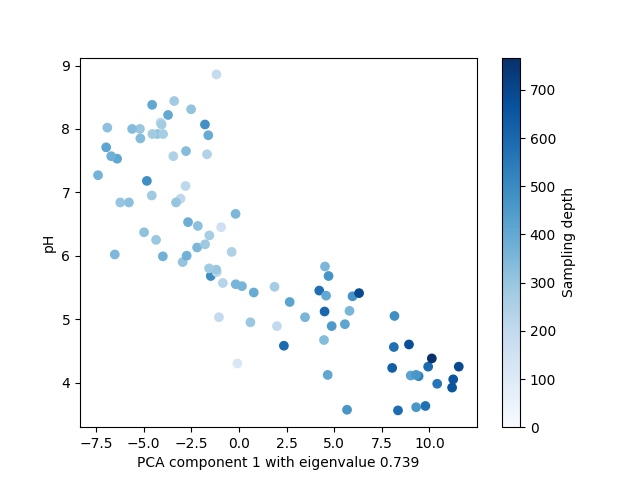
Spearman correlation between pH and 1st component: -0.8599836576738641, p-value: 3.777130551783766e-27

Temperature vs. PCA2

fig, ax = plt.subplots(1,1)
im = ax.scatter(proj[:,1], temperature, c = depth, cmap = plt.cm.Blues, vmin = 0)
cbar = fig.colorbar(im)
cbar.set_label("Sampling depth")
ax.set_xlabel(f"PCA component 2 with eigenvalue {eigv[1]}")
ax.set_ylabel("Temperature")


print("Spearman correlation between temperature and 2nd component: {0}, p-value: {1}".format(stats.spearmanr(temperature, proj[:,1])[0],
                                                                              stats.spearmanr(temperature, proj[:,1])[1]))

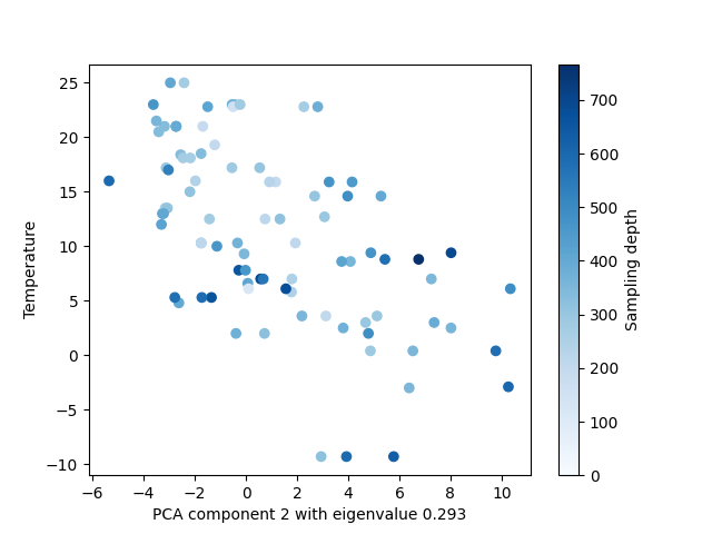
Spearman correlation between temperature and 2nd component: -0.5900116855285238, p-value: 1.1690533739643573e-09

We see that the projection of the sample data onto the low-rank components of Graphical Lasso is highly correlated to environmental confounders.