Note
Go to the end to download the full example code.
Benchmarking
We compare the performance of the Graphical Lasso solvers implemented in GGLasso to two commonly used packages, i.e.
regain : contains an ADMM solver which is doing almost the same operations as
ADMM_SGL. For details, see the original paper. [ref3]sklearn: by default uses the coordinate descent algorithm which was originally proposed by Friedman et al. [ref1]
The results can be generated using the notebook in benchmarks/benchmarks.ipynb in the Github repository.
From GGLasso we use the standard solver ADMM_SGL labeled by gglasso and the block-wise solver labeled by gglasso-block. For details, we refer to SGL solver.
import pandas as pd
import numpy as np

from gallery_helper import plot_bm
Synthetic power-law networks
We compare the solvers for a SGL problem using synthetic sparse powerlaw networks, which are generated as described in [ref2]. The solvers are tested for different values of \(\lambda_1\) and different dimensionalities. These values are printed below. We solve a SGL problem using each of the solvers independently, but using the same CPUs with 64GB of RAM in total.
The results were generated on a machine equipped with AMD Opteron(tm) 6378 @ 1.40GHz (max 2.40 GHz) (8 Cores per socket, hyper-threading).
df = pd.read_csv("../data/synthetic/bm5000.csv", index_col = 0)
df.reset_index(drop=True)
all_p_N = sorted(list(set(zip(df['p'], df['N']))))
print("Dimensionality and sample size: (p,N) =", all_p_N )

all_l1 = pd.unique(df.l1)
print("Values of lambda_1:  =", all_l1 )
Dimensionality and sample size: (p,N) = [(500, 550), (1000, 1100), (2000, 2200), (4000, 4400), (5000, 5500)]
Values of lambda_1:  = [0.05 0.1  0.5 ]
Setup
Each solver terminates after a given number of maximum iterations or when some optimality condition is met. Hence, the performance is difficult to compare as these optimality criteria may differ.
Thus, we select a range of values for relative (rtol) and absolute (tol) tolerance (used in ADMM) and similarly tolerance values for sklearn.
Calculating the accuracy
After solving each of the problems which each solver for different tolerance values, we compare the obtained solutions to a reference solution, denoted by \(Z^\ast\).
\(Z^\ast\) is obtained by solving a SGL problem by one of the solvers for very small tolerance values (we used regain and set tol=rtol=1e-10).
Finally, for a solution \(Z\), we calculate its accuracy using the normalized Euclidean distance:
Runtime and accuracy with respect to \(\lambda_1\).
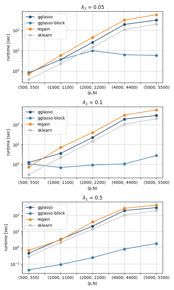
Now, determine a maximal accuracy \(\epsilon\). For each solver, we now select the run with minimal runtime where \(\text{accuracy}(Z) \leq \epsilon\) is fulfilled. We plot the results for two values of \(\epsilon\):
Accuracy of \(\epsilon=5\cdot10^{-3}\)
plot_bm(df, min_acc= 5e-3, lambda_list=all_l1)
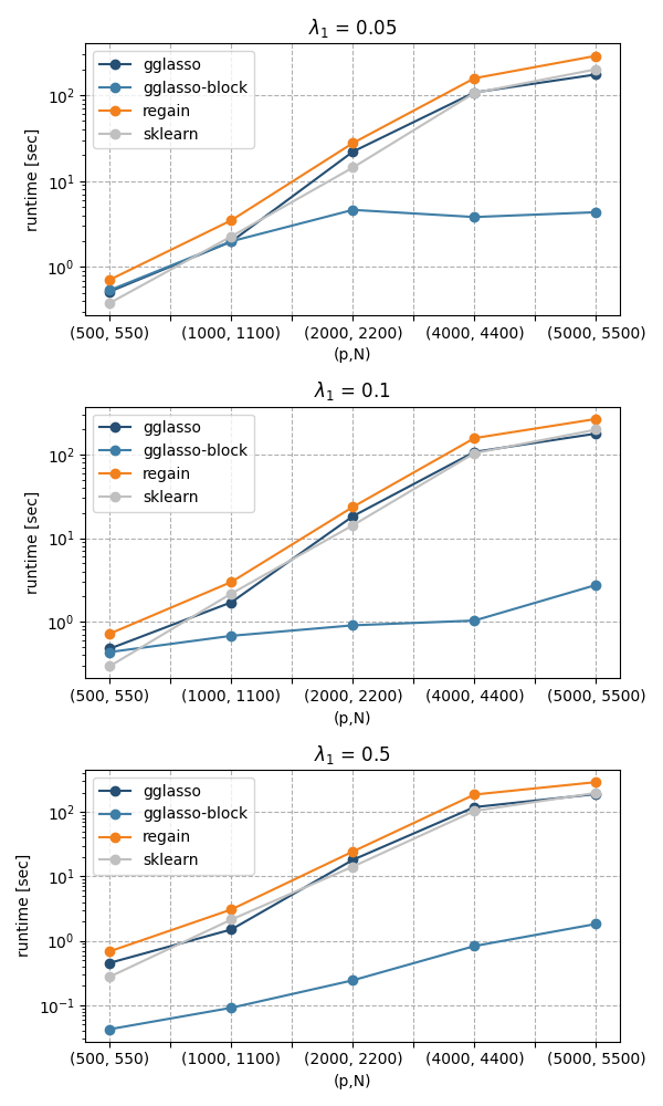
Accuracy of \(\epsilon=5\cdot10^{-2}\)
plot_bm(df, min_acc = 5e-2, lambda_list=all_l1)
Total running time of the script: (0 minutes 1.610 seconds)