Mathematical description

The GGLasso package can solve several problem formulations related to Graphical Lasso. On this page, we aim to define the exact formulation for each problem.

Single Graphical Lasso problems (SGL)

Consider a multivariate Gaussian variable

\[\mathcal{X} \sim \mathcal{N}(\mu, \Sigma) \in \mathbb{R}^p\]

Zeros in the precision matrix, \(\Sigma^{-1}\) correspond to conditional independence of two components of \(X\) which motivates a sparse estimation of \(\Sigma^{-1}\). Typically, we are given a sample of \(N\) independent samples of \(X\) for which we can compute the empirical covariance matrix \(S\). Even though \(S^{-1}\) (if exists) is the maximum-likelihood estimator of the precision matrix, it is not guaranteed to be sparse.

This leads to the nonsmooth convex optimization problem, known under the name of Graphical Lasso [ref1], given by

\[\min_{\Theta \in \mathbb{S}^p_{++}} - \log \det \Theta + \mathrm{Tr}(S\Theta) + \lambda \|\Theta\|_{1,od}\]

where \(\mathbb{S}^p_{++}\) is the cone of symmetric positive definite matrices of size \(p \times p\), \(\|\cdot\|_{1,od}\) is the sum of absolute values of all off-diagonal elements and \(\mathrm{Tr}\) is the trace of a matrix.

SGL with latent variables

In presence of latent variables, the precision matrix of the marginal of observable variables turns out to have the structure sparse - low rank [ref4].

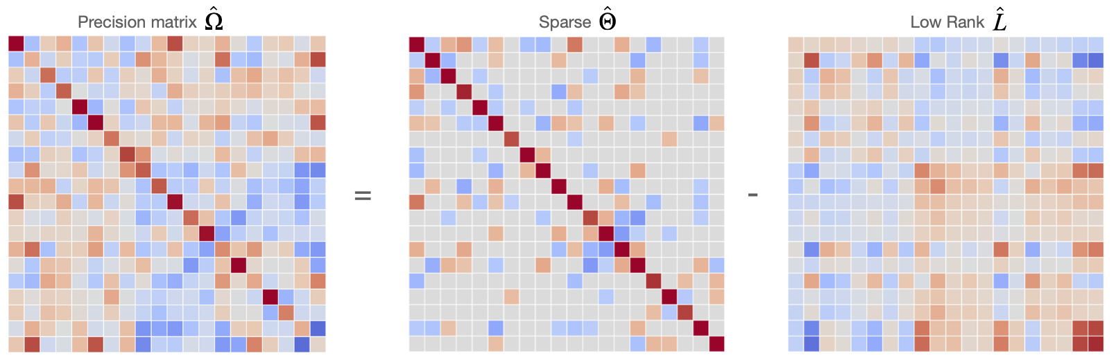
The problem can then be formulated as

\[\min_{\Theta, L \in \mathbb{S}^p} - \log \det (\Theta -L) + \mathrm{Tr}(S(\Theta-L)) + \lambda_1 \|\Theta\|_{1,od} + \mu_1 \|L\|_{\star}\]

where \(\|\cdot\|_{\star}\) is the nuclear norm (sum of singular values). \(\Theta\) represents the sparse part while \(L\) encodes the low rank component. In [ref12], latent variable Graphical Lasso has been studied in the context of microbial abundance analysis and microbiome interaction networks.

Multiple Graphical Lasso problems (MGL)

In many applications, observations of the same variables but coming from different distributions or in a temporal context are available. For example, consider gene expression data coming from cancer tissue samples and normal tissue samples [ref2]. Hence, there has been an increased interest in estimating precision matrices for multiple instances jointly [ref2], [ref3]. Mathematically, we consider \(K\) Gaussians

\[\mathcal{X}^{(k)} \sim \mathcal{N}(\mu^{(k)}, \Sigma^{(k)})\in \mathbb{R}^{p}.\]

Group Graphical Lasso (GGL) describes the problem of estimating precision matrices across multiple instances of the same class under the assumption that the sparsity patterns are similar. On the other hand, for time-varying data Fused Graphical Lasso was designed in order to get time-consistent estimates of the precision matrices, i.e. \(K\) is the temporal index.

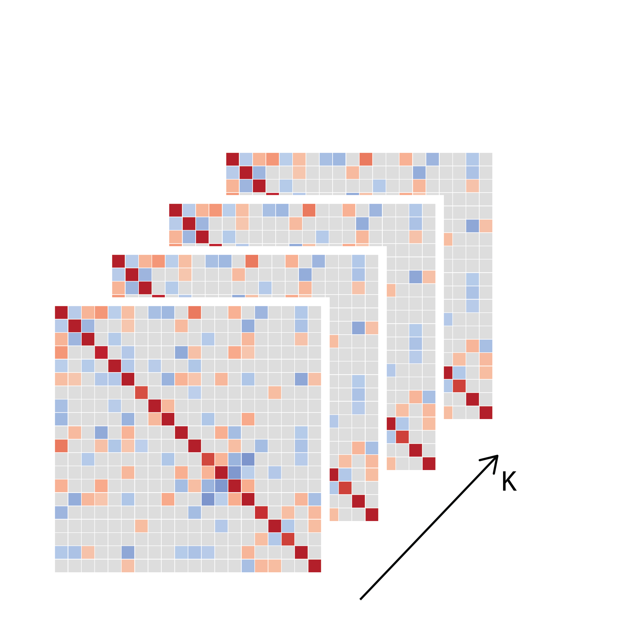
More generally, the problem formulation of Multiple Graphical Lasso is given by

\[\min_{\Theta}\quad \sum_{k=1}^{K} \left(-\log\det(\Theta^{(k)}) + \langle S^{(k)}, \Theta^{(k)} \rangle \right)+ \mathcal{P}(\Theta).\]

In the above, the feasible set is the \(K\)-fold product of \(\mathbb{S}^p_{++}\), see an illustration below. We denote an element of this space \(\Theta = (\Theta^{(1)}, \dots , \Theta^{(K)})\). As input, we have the empirical covariance matrices \(S = (S^{(1)}, \dots , S^{(K)})\) given.

Group Graphical Lasso (GGL)

For the Group Graphical Lasso problem, the regularization function is given by

\[\mathcal{P}(\Theta) = \lambda_1 \sum_{k=1}^{K} \sum_{i \neq j} |\Theta_{ij}^{(k)}| + \lambda_2 \sum_{i \neq j} \left(\sum_{k=1}^{K} |\Theta_{ij}^{(k)}|^2 \right)^{\frac{1}{2}}\]

with positive numbers \(\lambda_1, \lambda_2\). The first term promotes off-diagonal sparsity of the estimator while the second term – similar to the classical group penalty – induces that the non-zero entries are present for all instances \(\Theta^{(k)}\).

Fused Graphical Lasso (FGL)

For the Fused Graphical Lasso problem, the regularization function is given by

\[\mathcal{P}(\Theta) = \lambda_1 \sum_{k=1}^{K} \sum_{i \neq j} |\Theta_{ij}^{(k)}| + \lambda_2 \sum_{k=2}^{K} \sum_{i \neq j} |\Theta_{ij}^{(k)} - \Theta_{ij}^{(k-1)}|\]

with positive numbers \(\lambda_1, \lambda_2\). The first term promotes off-diagonal sparsity of the estimator while the second term – also known as total-variation penalty – induces that subsequent estimates of \(\Theta^{(k)}\) are similar.

MGL with latent variables

Analogous to SGL, we can extend MGL problems with latent variables. The problem formulation then becomes

\[\min_{\Theta, L}\quad \sum_{k=1}^{K} \left(-\log\det(\Theta^{(k)}- L^{(k)}) + \langle S^{(k)}, \Theta^{(k)} - L^{(k)} \rangle \right)+ \mathcal{P}(\Theta) +\sum_{k=1}^{K} \mu_{1,k} \|L^{(k)}\|_{\star}.\]

Software is already available for FGL (with and without latent variables) in [ref3], however also the deviation of the low rank matrices is included in the penalty.

GGL - the nonconforming case

So far, we have assumed that each component of \(\mathcal{X}^{(k)}\) is present in each of the \(K\) instances. However, in many practical situations this will not be the case. For example, assume that we have \(K\) datasets of microbiome abundances but not every microbiome species (OTU) was measured in each dataset. Hence, we may want to estimate the association network but with a group sparsity penalty on all overlapping pairs of species.

Consequently, assume that we have \(\mathcal{X}^{(k)} \sim \mathcal{N}(\mu^{(k)}, \Sigma^{(k)})\in \mathbb{R}^{p_k}\) and that there exist groups of overlapping pairs of variables \(G_1, \dots, G_L\) with

\[G_l = \{(i_l^k, j_l^k) \in \mathbb{N}^2 \vert k \in K_l \}, \quad K_l \subset K\]

where \(k \in K_l\) if and only if the pair of variables corresponding to \(G_l\) exists in \(\mathcal{X}^{(k)}\). In that case \((i_l^k, j_l^k)\) are the indices of the relevant entry in \(\Theta^{(k)}\) for group \(l\).

Now, the associated GGL regularizer becomes

\[\mathcal{P}(\Theta) = \lambda_1 \sum_{i \neq j, k} |\Theta_{ij}^{(k)}| + \lambda_2 \sum_{l=1}^{L}\beta_l \|\Theta_{[l]}\|\]

where \(\Theta_{[l]}\) is the vector with entries \(\{\Theta_{i_l^k j_l^k}^{(k)} \vert~ k \in K_l\} \in \mathbb{R}^{|K_l|}\). The scaling factor \(\beta_l > 0\) is set to \(\beta_l = \sqrt{|K_l|}\) in order to account for distinct group sizes.

In GGLasso we implemented an ADMM algorithm for the above described problem formulation, possibly extended with latent variables. Have a look at the Nonconforming Group Graphical Lasso experiment in our example gallery.

Functional Graphical Lasso

Functional Graphical Lasso is a variant of Single Graphical Lasso, where each variable is not represented as a scalar, but as a function (or time series) [ref13]. Hence, assume that each variable has a \(M\)-dimensional representation, for example coming from Functional PCA, Fourier transform or using a spline basis. Functional Graphical Lasso can be understood as SGL but with each matrix entry being an \(M\times M\) block, representing the association between two function variables. Therefore, the regularization results in each \(M\times M\) block either being zero or non-zero, and typically being dense in the latter case.

For \(p\) variables, we compute the covariance matrix \(S \in \mathbb{R}^{pM\times pM}\). The problem formulation is

\[\min_{\Theta \in \mathbb{S}^{p\cdot M}_{++}} - \log \det \Theta + \mathrm{Tr}(S\Theta) + \lambda_1 \sum_{j\neq l} \|\Theta_{jl}^M\|_{F}.\]

With latent variables, our implementation solves

\[\min_{\Theta, L \in \mathbb{S}^{p\cdot M}_{++}} - \log \det (\Theta -L) + \mathrm{Tr}(S (\Theta -L)) + \lambda_1 \sum_{j\neq l} \|\Theta_{jl}^M\|_{F} + \mu_1 \|L\|_{\star}.\]

We have a simple tutorial on this in the Functional Graphical Lasso experiment.

Optimization algorithms

All of the above problem formulations are instances of nonlinear, convex and nonsmooth optimization problems. See Algorithms for an overview of solvers which we implemented for these problems and a short guide on how to use them.

References

[ref1]

Friedman, J., Hastie, T., and Tibshirani, R. (2007). Sparse inverse covariance estimation with the Graphical Lasso. Biostatistics, 9(3):432–441.

[ref2] (1,2)

Danaher, P., Wang, P., and Witten, D. M. (2013). The joint graphical lasso for inverse covariance estimation across multiple classes. Journal of the Royal Statistical Society: Series B (Statistical Methodology), 76(2):373–397.

[ref3] (1,2)

Tomasi, F., Tozzo, V., Salzo, S., and Verri, A. (2018). Latent Variable Time-varying Network Inference. InProceedings of the 24th ACM SIGKDD International Conference on Knowledge Discovery & Data Mining. ACM.

[ref4]

Chandrasekaran, V., Parrilo, P. A., and Willsky, A. S. (2012). Latent variable graphical model selection via convex optimization. The Annals of Statistics, 40(4):1935–1967.

[ref5]

Ma, S., Xue, L., and Zou, H. (2013). Alternating Direction Methods for Latent Variable Gaussian Graphical Model Selection. Neural Computation, 25(8):2172–2198.

[ref6]

Zhang, Y., Zhang, N., Sun, D., and Toh, K.-C. (2020). A proximal point dual Newton algorithm for solving group graphical Lasso problems. SIAM J. Optim., 30(3):2197–2220.

[ref7]

Zhang, N., Zhang, Y., Sun, D., and Toh, K.-C. (2019). An efficient linearly convergent regularized proximal point algorithm for fused multiple graphical lasso problems.

[ref8]

Boyd, S., Parikh, N., Chu, E., Peleato, B., and Eckstein, J. (2011). Distributed Optimization and Statistical Learning via the Alternating Direction Method of Multipliers. Found. Trends Mach. Learn., 3(1):1–122.

[ref9]

Witten, D. M., Friedman, J. H., and Simon, N. (2011). New Insights and Faster Computations for the Graphical Lasso. J. Comput. Graph. Statist., 20(4):892–900.

[ref10]

Foygel, R. and Drton, M. (2010). Extended Bayesian Information Criteria for Gaussian Graphical Models. In Lafferty, J., Williams, C., Shawe-Taylor, J.,Zemel, R., and Culotta, A., editors, Advances in Neural Information Processing Systems, volume 23. Curran Associates, Inc.

[ref11]

Condat, L. (2013). A Direct Algorithm for 1-D Total Variation Denoising, IEEE Signal Processing Letters, vol. 20, no. 11, pp. 1054-1057.

[ref12]

Kurtz, Z. D., Bonneau, R., and Mueller, C. L. (2019). Disentangling microbial associations from hidden environmental and technical factors via latent graphical models.

[ref13]

Qiao, X., Guo, S., and James, G. M. (2019) Functional graphical models, J. Amer. Statist. Assoc., 114, 211-222.