Fused Graphical Lasso experiment

We investigate the performance of Fused Graphical Lasso on powerlaw networks, compared to estimating the precision matrices independently with SGL. In particular, we demonstrate that FGL - in contrast to SGL - is capable of estimating time-consistent precision matrices.

We generate a precision matrix with block-wise powerlaw networks. At time K=5, one of the blocks disappears and another block appears. A third block decays exponentially over time (indexed by K).

# sphinx_gallery_thumbnail_number = 2

import numpy as np
from sklearn.covariance import GraphicalLasso
from regain.covariance import TimeGraphicalLasso

from gglasso.solver.admm_solver import ADMM_MGL
from gglasso.helper.data_generation import time_varying_power_network, sample_covariance_matrix
from gglasso.helper.experiment_helper import discovery_rate, error
from gglasso.helper.utils import get_K_identity
from gglasso.helper.experiment_helper import plot_evolution, plot_deviation, surface_plot, single_heatmap_animation
from gglasso.helper.model_selection import aic, ebic


p = 100
K = 10
N = 5000
M = 5
L = int(p/M)

reg = 'FGL'

Sigma, Theta = time_varying_power_network(p, K, M, scale = False, seed = 2340)

S, sample = sample_covariance_matrix(Sigma, N)


results = {}
results['truth'] = {'Theta' : Theta}

Animate precision matrix over time

colored squares represent non-zero entries

anim = single_heatmap_animation(Theta)

Once Loop Reflect

Parameter selection (FGL)

We do a grid search over \(\lambda_1\) and \(\lambda_2\) values. On each grid point we evaluate True/False Discovery Rate (TPR/FPR), True/False Discovery of Differential edges and AIC and eBIC.

Note: the package contains functions for doing this grid search, but here we also want to evaluate True and False positive rates on each grid points.

l2 = 2*np.logspace(start = -1, stop = -3, num = 5, base = 10)
l1 = 2*np.logspace(start = -1, stop = -3, num = 10, base = 10)
L2, L1 = np.meshgrid(l2,l1)
grid1 = L1.shape[0]; grid2 = L2.shape[1]

ERR = np.zeros((grid1, grid2))
FPR = np.zeros((grid1, grid2))
TPR = np.zeros((grid1, grid2))
DFPR = np.zeros((grid1, grid2))
DTPR = np.zeros((grid1, grid2))
AIC = np.zeros((grid1, grid2))
BIC = np.zeros((grid1, grid2))

Omega_0 = get_K_identity(K,p)
Theta_0 = get_K_identity(K,p)
X_0 = np.zeros((K,p,p))

for g2 in np.arange(grid2):
    for g1 in np.arange(grid1):

        lambda1 = L1[g1,g2]
        lambda2 = L2[g1,g2]

        sol, info =  ADMM_MGL(S, lambda1, lambda2, reg , Omega_0, Theta_0 = Theta_0, X_0 = X_0, tol = 1e-8, rtol = 1e-8, verbose = False, measure = False)

        Theta_sol = sol['Theta']
        Omega_sol = sol['Omega']
        X_sol = sol['X']

        # warm start
        Omega_0 = Omega_sol.copy()
        Theta_0 = Theta_sol.copy()
        X_0 = X_sol.copy()

        dr = discovery_rate(Theta_sol, Theta)
        TPR[g1,g2] = dr['TPR']
        FPR[g1,g2] = dr['FPR']
        DTPR[g1,g2] = dr['TPR_DIFF']
        DFPR[g1,g2] = dr['FPR_DIFF']
        ERR[g1,g2] = error(Theta_sol, Theta)
        AIC[g1,g2] = aic(S, Theta_sol, N)
        BIC[g1,g2] = ebic(S, Theta_sol, N, gamma = 0.1)


# get optimal lambda
ix= np.unravel_index(np.nanargmin(BIC), BIC.shape)
ix2= np.unravel_index(np.nanargmin(AIC), AIC.shape)

l1opt = L1[ix]
l2opt = L2[ix]

print("Optimal lambda values: (l1,l2) = ", (l1opt,l2opt))

ADMM terminated after 46 iterations with status: optimal.
ADMM terminated after 43 iterations with status: optimal.
ADMM terminated after 42 iterations with status: optimal.
ADMM terminated after 43 iterations with status: optimal.
ADMM terminated after 43 iterations with status: optimal.
ADMM terminated after 44 iterations with status: optimal.
ADMM terminated after 44 iterations with status: optimal.
ADMM terminated after 44 iterations with status: optimal.
ADMM terminated after 43 iterations with status: optimal.
ADMM terminated after 43 iterations with status: optimal.
ADMM terminated after 44 iterations with status: optimal.
ADMM terminated after 42 iterations with status: optimal.
ADMM terminated after 42 iterations with status: optimal.
ADMM terminated after 43 iterations with status: optimal.
ADMM terminated after 41 iterations with status: optimal.
ADMM terminated after 44 iterations with status: optimal.
ADMM terminated after 44 iterations with status: optimal.
ADMM terminated after 41 iterations with status: optimal.
ADMM terminated after 43 iterations with status: optimal.
ADMM terminated after 43 iterations with status: optimal.
ADMM terminated after 45 iterations with status: optimal.
ADMM terminated after 42 iterations with status: optimal.
ADMM terminated after 42 iterations with status: optimal.
ADMM terminated after 42 iterations with status: optimal.
ADMM terminated after 42 iterations with status: optimal.
ADMM terminated after 41 iterations with status: optimal.
ADMM terminated after 41 iterations with status: optimal.
ADMM terminated after 22 iterations with status: optimal.
ADMM terminated after 21 iterations with status: optimal.
ADMM terminated after 19 iterations with status: optimal.
ADMM terminated after 43 iterations with status: optimal.
ADMM terminated after 41 iterations with status: optimal.
ADMM terminated after 43 iterations with status: optimal.
ADMM terminated after 41 iterations with status: optimal.
ADMM terminated after 37 iterations with status: optimal.
ADMM terminated after 20 iterations with status: optimal.
ADMM terminated after 21 iterations with status: optimal.
ADMM terminated after 16 iterations with status: optimal.
ADMM terminated after 14 iterations with status: optimal.
ADMM terminated after 14 iterations with status: optimal.
ADMM terminated after 45 iterations with status: optimal.
ADMM terminated after 42 iterations with status: optimal.
ADMM terminated after 42 iterations with status: optimal.
ADMM terminated after 41 iterations with status: optimal.
ADMM terminated after 32 iterations with status: optimal.
ADMM terminated after 22 iterations with status: optimal.
ADMM terminated after 16 iterations with status: optimal.
ADMM terminated after 15 iterations with status: optimal.
ADMM terminated after 15 iterations with status: optimal.
ADMM terminated after 15 iterations with status: optimal.
Optimal lambda values: (l1,l2) =  (0.02583099330029768, 0.06324555320336758)

Solving time-varying problems with SGL

We now solve K independent SGL problems and find the best \(\lambda_1\) parameter.

ALPHA = 2*np.logspace(start = -3, stop = -1, num = 10, base = 10)
SGL_BIC = np.zeros(len(ALPHA))
all_res = list()

for j in range(len(ALPHA)):
    res = np.zeros((K,p,p))
    singleGL = GraphicalLasso(alpha = ALPHA[j], tol = 1e-3, max_iter = 20, verbose = False)
    for k in np.arange(K):
        model = singleGL.fit(sample[k,:,:].T)
        res[k,:,:] = model.precision_

    all_res.append(res)
    SGL_BIC[j] = ebic(S, res, N, gamma = 0.1)

ix_SGL = np.argmin(SGL_BIC)
results['SGL'] = {'Theta' : all_res[ix_SGL]}

Solve with ADMM

Omega_0 = get_K_identity(K,p)

sol, info = ADMM_MGL(S, l1opt, l2opt, reg, Omega_0, rho = 1, max_iter = 500, \
                                                        tol = 1e-10, rtol = 1e-10, verbose = False, measure = True)


results['ADMM'] = {'Theta' : sol['Theta']}

ADMM terminated after 92 iterations with status: optimal.

Solve with regain

regain needs data in format (N*K,p). regain includes the TV penalty also on the diagonal, hence results may be slightly different than ADMM_MGL.

tmp = sample.transpose(1,0,2).reshape(p,-1).T


ltgl = TimeGraphicalLasso(alpha = N*l1opt, beta = N*l2opt  , psi = 'l1', \
                          rho = 1., tol = 1e-10, rtol = 1e-10,  max_iter = 500, verbose = False)
ltgl = ltgl.fit(X = tmp, y = np.repeat(np.arange(K),N))



results['LTGL'] = {'Theta' : ltgl.precision_}

Plotting: deviation, eBIC surface, recovery

Description of plots:

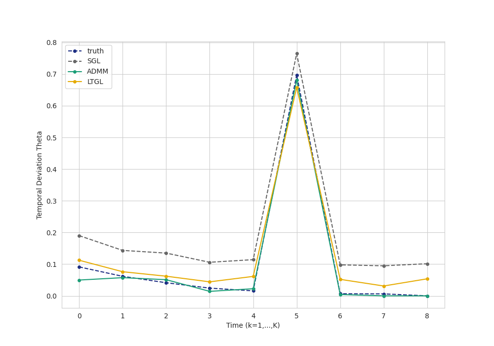
1. Deviation of subsequent precision matrices: SGL varies heavily over time while FGL is able to recover the true deviation quite well.

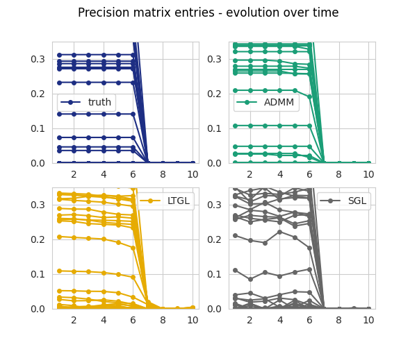
2. Plot each entry of the disappearing block over time (one line = one precision matrix entry)

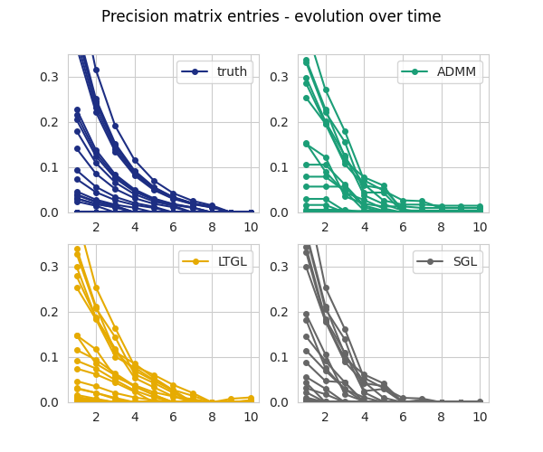
3. Plot each entry of the exponentially decaying block over time (one line = one precision matrix entry)

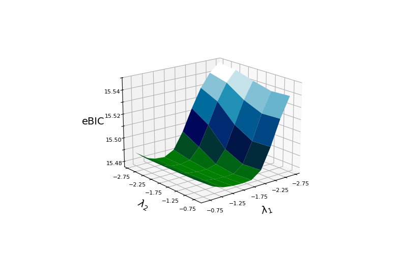
4. Surface plot of eBIC over the grid of \(\lambda_1\) and \(\lambda_2\).

Theta_admm = results.get('ADMM').get('Theta')
Theta_ltgl = results.get('LTGL').get('Theta')
Theta_sgl = results.get('SGL').get('Theta')



print("Norm(Regain-ADMM)/Norm(ADMM):", np.linalg.norm(Theta_ltgl - Theta_admm)/ np.linalg.norm(Theta_admm))


plot_deviation(results)

plot_evolution(results, block = 0, L = L)

plot_evolution(results, block = 2, L = L)

fig = surface_plot(L1, L2, BIC, name = 'eBIC')

• 
• 
• 
• 

Norm(Regain-ADMM)/Norm(ADMM): 0.03290781887376122